Systems of differential equations, methods of integration. How to solve a system of differential equations using the operational method? Particular solutions of a system of differential equations

Many systems of differential equations, both homogeneous and inhomogeneous, can be reduced to one equation for one unknown function. Let's demonstrate the method with examples.

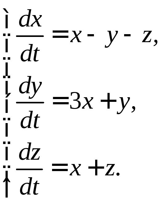
Example 3.1. Solve the system

Solution. 1) Differentiating by t first equation and using the second and third equations to replace And , we find

We differentiate the resulting equation with respect to again

1) We create a system

From the first two equations of the system we express the variables And through
:

Let us substitute the found expressions for And into the third equation of the system

So, to find the function
obtained a third order differential equation with constant coefficients

.

2) We integrate the last equation using the standard method: we compose the characteristic equation
, find its roots
and construct a general solution in the form of a linear combination of exponentials, taking into account the multiplicity of one of the roots:.

3) Next to find the two remaining functions
And
, we differentiate the resulting function twice

Using connections (3.1) between the functions of the system, we recover the remaining unknowns

.

Answer. ,
,.

It may turn out that all known functions except one are excluded from the third-order system even with a single differentiation. In this case, the order of the differential equation for finding it will be less than the number of unknown functions in the original system.

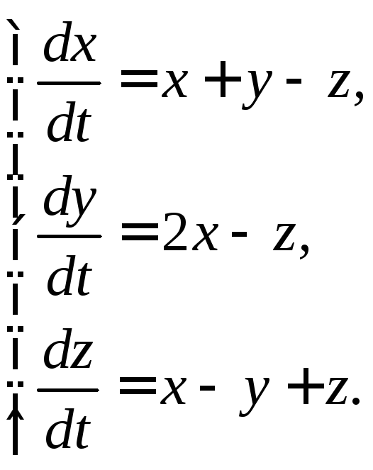
Example 3.2. Integrate the system

(3.2)

Solution. 1) Differentiating by the first equation, we find

Excluding Variables And from equations

we will have a second order equation with respect to

(3.3)

2) From the first equation of system (3.2) we have

(3.4)

Substituting into the third equation of system (3.2) the found expressions (3.3) and (3.4) for And , we obtain a first order differential equation to determine the function

Integrating this inhomogeneous equation with constant first-order coefficients, we find
Using (3.4), we find the function

Answer.
,,
.

Task 3.1. Solve homogeneous systems by reducing them to one differential equation.

3.1.1. 3.1.2.

3.1.3. 3.1.4.

3.1.5. 3.1.6.

3.1.7. 3.1.8.

3.1.9. 3.1.10.

3.1.11. 3.1.12.

3.1.13. 3.1.14.

3.1.15. 3.1.16.

3.1.17. 3.1.18.

3.1.19. 3.1.20.

3.1.21. 3.1.22.

3.1.23. 3.1.24.

3.1.25. 3.1.26.

3.1.27. 3.1.28.

3.1.29.
3.1.30.

3.2. Solving systems of linear homogeneous differential equations with constant coefficients by finding a fundamental system of solutions

The general solution to a system of linear homogeneous differential equations can be found as a linear combination of the fundamental solutions of the system. In the case of systems with constant coefficients, linear algebra methods can be used to find fundamental solutions.

Example 3.3. Solve the system

(3.5)

Solution. 1) Let's rewrite the system in matrix form

. (3.6)

2) We will look for a fundamental solution of the system in the form of a vector
. Substituting functions
in (3.6) and reducing by , we get

, (3.7)

that is the number must be an eigenvalue of the matrix
, and the vector the corresponding eigenvector.

3) From the course of linear algebra it is known that system (3.7) has a non-trivial solution if its determinant is equal to zero

,

that is . From here we find the eigenvalues
.

4) Find the corresponding eigenvectors. Substituting the first value into (3.7)
, we obtain a system for finding the first eigenvector

From here we get the connection between the unknowns
. It is enough for us to choose one non-trivial solution. Believing
, Then
, that is, the vector is eigenof eigenvalue
, and the function vector
fundamental solution of a given system of differential equations (3.5). Similarly, when substituting the second root
in (3.7) we have a matrix equation for the second eigenvector
. Where do we get the connection between its components?
. Thus, we have the second fundamental solution

.

5) The general solution of system (3.5) is constructed as a linear combination of the two obtained fundamental solutions

or in coordinate form

.

Answer.

.

Task 3.2. Solve systems by finding the fundamental system of solutions.

A system of this type is called normal system of differential equations (SNDU). For a normal system of differential equations, we can formulate a theorem on existence and uniqueness, the same as for a differential equation.

Theorem. If the functions are defined and continuous on an open set, and the corresponding partial derivatives are also continuous on, then system (1) will have a solution (2)

and in the presence of initial conditions (3)

this solution will be the only one.

This system can be represented as:

Systems of linear differential equations

Definition. The system of Differential Equations is called linear , if it is linear with respect to all unknown functions and their derivatives.

(5)

General view of the system of Differential Equations

If the initial condition is given: , (7)

then the solution will be unique, provided that the vector function is continuous and the matrix coefficients are also continuous functions.

Let us introduce a linear operator, then (6) can be rewritten as:

if then the operator equation (8) is called homogeneous and has the form:

Since the operator is linear, the following properties are satisfied for it:

solving equation (9).

Consequence. Linear combination, solution (9).

If solutions (9) are given and they are linearly independent, then all linear combinations of the form: (10) only under the condition that all. This means that the determinant composed of solutions (10):

. This determinant is called Vronsky's determinant for a system of vectors.

Theorem 1. If the Wronski determinant for a linear homogeneous system (9) with coefficients continuous on an interval is equal to zero at least at one point, then the solutions are linearly dependent on this interval and, therefore, the Wronski determinant is equal to zero on the entire interval.

Proof: Since they are continuous, system (9) satisfies the condition Existence and uniqueness theorems, therefore, the initial condition determines the unique solution of system (9). The Wronski determinant at a point is equal to zero, therefore, there is a non-trivial system for which the following holds: The corresponding linear combination for another point will have the form, and satisfies homogeneous initial conditions, therefore, coincides with the trivial solution, that is, linearly dependent and the Wronski determinant is equal to zero.

Definition. The set of solutions of system (9) is called fundamental system of solutions on if the Wronski determinant does not vanish at any point.

Definition. If for a homogeneous system (9) the initial conditions are defined as follows - then the system of solutions is called normal fundamental decision system .

Comment. If is a fundamental system or a normal fundamental system, then the linear combination is the general solution (9).

Theorem 2. A linear combination of linearly independent solutions of a homogeneous system (9) with coefficients continuous on an interval will be a general solution (9) on the same interval.

Proof: Since the coefficients are continuous on, the system satisfies the conditions of the existence and uniqueness theorem. Therefore, to prove the theorem, it is enough to show that by selecting constants, it is possible to satisfy some arbitrarily chosen initial condition (7). Those. can be satisfied by the vector equation:. Since is a general solution to (9), the system is relatively solvable, since and are all linearly independent. We define it uniquely, and since we are linearly independent, then.

Theorem 3. If this is a solution to system (8), a solution to system (9), then + there will also be a solution to (8).

Proof: According to the properties of the linear operator: 

Theorem 4. The general solution (8) on an interval with coefficients and right-hand sides continuous on this interval is equal to the sum of the general solution of the corresponding homogeneous system (9) and the particular solution of the inhomogeneous system (8).

Proof: Since the conditions of the theorem on existence and uniqueness are satisfied, therefore, it remains to prove that it will satisfy an arbitrarily given initial value (7), that is . (11)

For system (11) it is always possible to determine the values ​​of . This can be done as a fundamental decision system.

Cauchy problem for a first order differential equation

Formulation of the problem. Recall that the solution to a first-order ordinary differential equation

y"(t)=f(t, y(t)) (5.1)

is called a differentiable function y(t), which, when substituted into equation (5.1), turns it into an identity. The graph of the solution to a differential equation is called an integral curve. The process of finding solutions to a differential equation is usually called integrating this equation.

Based on the geometric meaning of the derivative y", we note that equation (5.1) specifies at each point (t, y) in the plane of variables t, y the value f(t, y) of the tangent of the angle of inclination (to the 0t axis) of the tangent to the graph of the solution passing through This point. The quantity k=tga=f(t,y) will be called the angular coefficient (Fig. 5.1). If now at each point (t,y) we specify the direction of the tangent, determined by the value f(t,y), using a certain vector. ), then we get the so-called direction field (Fig. 5.2, a). Thus, geometrically, the task of integrating differential equations is to find integral curves that at each point have a given tangent direction (Fig. 5.2, b). to select one specific solution from the family of solutions of the differential equation (5.1), set the initial condition

y(t 0)=y 0 (5.2)

Here t 0 is some fixed value of the argument t, and 0 has a value called the initial value. The geometric interpretation of using the initial condition is to select from a family of integral curves the curve that passes through a fixed point (t 0, y 0).

The problem of finding for t>t 0 a solution y(t) to the differential equation (5.1) satisfying the initial condition (5.2) will be called the Cauchy problem. In some cases, the behavior of the solution for all t>t 0 is of interest. However, more often they are limited to determining the solution on a finite segment.

Integration of normal systems

One of the main methods for integrating a normal DE system is the method of reducing the system to one higher order DE. (The inverse problem - the transition from the remote control to the system - was considered above using an example.) The technique of this method is based on the following considerations.

Let a normal system (6.1) be given. Let's differentiate any equation, for example the first one, with respect to x:

Substituting into this equality the values ​​of the derivatives from system (6.1), we obtain

or, briefly,

Differentiating the resulting equality again and replacing the values ​​of the derivatives from system (6.1), we obtain

Continuing this process (differentiate - substitute - get), we find:

Let's collect the resulting equations into a system:

From the first (n-1) equations of system (6.3) we express the functions y 2, y 3, ..., y n in terms of x, the function y 1 and its derivatives y" 1, y" 1,..., y 1 (n -1) . We get:

We substitute the found values ​​of y 2, y 3,..., y n into the last equation of system (6.3). Let us obtain one nth order DE with respect to the desired function. Let its general solution be

Differentiate it (n-1) times and substitute the values ​​of the derivatives into the equations of system (6.4), we find the functions y 2, y 3,..., y n.

Example 6.1. Solve system of equations

Solution: Let's differentiate the first equation: y"=4y"-3z". Substitute z"=2y-3z into the resulting equality: y"=4y"-3(2y-3z), y"-4y"+6y=9z. Let's create a system of equations:

From the first equation of the system we express z through y and y":

We substitute the z value into the second equation of the last system:

i.e. y""-y"-6y=0. We received one LOD of the second order. Solve it: k 2 -k-6=0, k 1 =-2, k 2 =3 and - general solution

equations Find the function z. We substitute the values ​​of y and into the expression z through y and y" (formula (6.5)). We obtain:

Thus, the general solution to this system of equations has the form

Comment. System of equations (6.1) can be solved by the method of integrable combinations. The essence of the method is that, through arithmetic operations, the equations of a given system are used to form so-called integrable combinations, i.e., easily integrable equations with respect to a new unknown function.

Let us illustrate the technique of this method with the following example.

Example 6.2. Solve the system of equations:

Solution: Let's add the given equations term by term: x"+y"=x+y+2, or (x+y)"=(x+y)+2. Let's denote x+y=z. Then we have z"=z+2 . We solve the resulting equation:

We got the so-called first integral of the system. From it you can express one of the sought functions through another, thereby reducing the number of sought functions by one. For example, Then the first equation of the system will take the form

Having found x from it (for example, using the substitution x=uv), we will also find y.

Comment. This system “allows” to form another integrable combination: Putting x - y = p, we have:, or Having two first integrals of the system, i.e. And it is easy to find (by adding and subtracting the first integrals) that

Linear operator, properties. Linear dependence and independence of vectors. Wronski determinant for the LDE system.

Linear differential operator and its properties. The set of functions having on the interval ( a , b ) no less n derivatives, forms a linear space. Consider the operator L n (y ), which displays the function y (x ), having derivatives, into a function having k - n derivatives:

Using an operator L n (y ) inhomogeneous equation (20) can be written as follows:

L n (y ) = f (x );

homogeneous equation (21) takes the form

L n (y ) = 0);

Theorem 14.5.2. Differential operator L n (y ) is a linear operator. Document follows directly from the properties of derivatives: 1. If C = const, then 2. Our further actions: first study how the general solution of the linear homogeneous equation (25) works, then the inhomogeneous equation (24), and then learn how to solve these equations. Let's start with the concepts of linear dependence and independence of functions on an interval and define the most important object in the theory of linear equations and systems - the Wronski determinant.

Vronsky's determinant. Linear dependence and independence of a system of functions.Def. 14.5.3.1. Function system y 1 (x ), y 2 (x ), …, y n (x ) is called linearly dependent on the interval ( a , b ), if there is a set of constant coefficients not equal to zero at the same time, such that the linear combination of these functions is identically equal to zero on ( a , b ): for. If equality for is possible only if, the system of functions y 1 (x ), y 2 (x ), …, y n (x ) is called linearly independent on the interval ( a , b ). In other words, the functions y 1 (x ), y 2 (x ), …, y n (x ) linearly dependent on the interval ( a , b ), if there is an equal to zero on ( a , b ) their non-trivial linear combination. Functions y 1 (x ),y 2 (x ), …, y n (x ) linearly independent on the interval ( a , b ), if only their trivial linear combination is identically equal to zero on ( a , b ). Examples: 1. Functions 1, x , x 2 , x 3 are linearly independent on any interval ( a , b ). Their linear combination - polynomial of degree - cannot have on ( a , b )more than three roots, so the equality = 0 for is possible only when. Example 1 is easily generalized to function system 1, x , x 2 , x 3 , …, x n . Their linear combination - a polynomial of degree - cannot have on ( a , b ) more n roots. 3. The functions are linearly independent on any interval ( a , b ), If . Indeed, if, for example, then the equality takes place at a single point .4. Function system is also linearly independent if the numbers k i (i = 1, 2, …, n ) are pairwise different, but direct proof of this fact is quite cumbersome. As the above examples show, in some cases the linear dependence or independence of functions is proven simply, in other cases this proof is more complicated. Therefore, a simple universal tool is needed that will answer the question about the linear dependence of functions. Such a tool - Vronsky's determinant.

Def. 14.5.3.2. Wronsky's determinant (Wronskian) systems n - 1 time differentiable functions y 1 (x ), y 2 (x ), …, y n (x ) is called the determinant

.

14.5.3.3. Theorem on the Wronskian of a linearly dependent system of functions. If the system of functions y 1 (x ), y 2 (x ), …, y n (x ) linearly dependent on the interval ( a , b ), then the Wronskian of this system is identically equal to zero on this interval. Document. If the functions y 1 (x ), y 2 (x ), …, y n (x ) are linearly dependent on the interval ( a , b ), then there are numbers , at least one of which is non-zero, such that

Let's differentiate by x equality (27) n - 1 time and create a system of equations We will consider this system as a homogeneous linear system of algebraic equations with respect to. The determinant of this system is the Wronski determinant (26). This system has a nontrivial solution, therefore, at each point its determinant is equal to zero. So, W (x ) = 0 at , i.e. at ( a , b ).

Matrix representation of a system of ordinary differential equations (SODE) with constant coefficients

Linear homogeneous SODE with constant coefficients $\left\(\begin(array)(c) (\frac(dy_(1) )(dx) =a_(11) \cdot y_(1) +a_(12) \cdot y_ (2) +\ldots +a_(1n) \cdot y_(n) \\ (\frac(dy_(2) )(dx) =a_(21) \cdot y_(1) +a_(22) \cdot y_(2) +\ldots +a_(2n) \cdot y_(n) ) \\ (\ldots ) \\ (\frac(dy_(n) )(dx) =a_(n1) \cdot y_(1) +a_(n2) \cdot y_(2) +\ldots +a_(nn) \cdot y_(n) ) \end(array)\right $,

where $y_(1)\left(x\right),\; y_(2)\left(x\right),\; \ldots ,\; y_(n) \left(x\right)$ -- the required functions of the independent variable $x$, coefficients $a_(jk) ,\; 1\le j,k\le n$ -- we represent the given real numbers in matrix notation:

1. matrix of required functions $Y=\left(\begin(array)(c) (y_(1) \left(x\right)) \\ (y_(2) \left(x\right)) \\ (\ldots ) \\ (y_(n) \left(x\right)) \end(array)\right)$;
2. matrix of derivative solutions $\frac(dY)(dx) =\left(\begin(array)(c) (\frac(dy_(1) )(dx) ) \\ (\frac(dy_(2) )(dx ) ) \\ (\ldots ) \\ (\frac(dy_(n) )(dx) ) \end(array)\right)$;
3. SODE coefficient matrix $A=\left(\begin(array)(cccc) (a_(11) ) & (a_(12) ) & (\ldots ) & (a_(1n) ) \\ (a_(21) ) & (a_(22) ) & (\ldots ) & (a_(2n) ) \\ (\ldots ) & (\ldots ) & (\ldots ) & (\ldots ) \\ (a_(n1) ) & ( a_(n2) ) & (\ldots ) & (a_(nn) ) \end(array)\right)$.

Now, based on the rule of matrix multiplication, this SODE can be written in the form of a matrix equation $\frac(dY)(dx) =A\cdot Y$.

General method for solving SODE with constant coefficients

Let there be a matrix of some numbers $\alpha =\left(\begin(array)(c) (\alpha _(1) ) \\ (\alpha _(2) ) \\ (\ldots ) \\ (\alpha _ (n) ) \end(array)\right)$.

The solution to the SODE is found in the following form: $y_(1) =\alpha _(1) \cdot e^(k\cdot x) $, $y_(2) =\alpha _(2) \cdot e^(k\ cdot x) $, \dots , $y_(n) =\alpha _(n) \cdot e^(k\cdot x) $. In matrix form: $Y=\left(\begin(array)(c) (y_(1) ) \\ (y_(2) ) \\ (\ldots ) \\ (y_(n) ) \end(array )\right)=e^(k\cdot x) \cdot \left(\begin(array)(c) (\alpha _(1) ) \\ (\alpha _(2) ) \\ (\ldots ) \\ (\alpha _(n) ) \end(array)\right)$.

From here we get:

Now the matrix equation of this SODE can be given the form:

The resulting equation can be represented as follows:

The last equality shows that the vector $\alpha $ using the matrix $A$ is transformed into a parallel vector $k\cdot \alpha $. This means that the vector $\alpha $ is an eigenvector of the matrix $A$, corresponding to the eigenvalue $k$.

The number $k$ can be determined from the equation $\left|\begin(array)(cccc) (a_(11) -k) & (a_(12) ) & (\ldots ) & (a_(1n) ) \\ ( a_(21) ) & (a_(22) -k) & (\ldots ) & (a_(2n) ) \\ (\ldots ) & (\ldots ) & (\ldots ) & (\ldots ) \\ ( a_(n1) ) & (a_(n2) ) & (\ldots ) & (a_(nn) -k) \end(array)\right|=0$.

This equation is called characteristic.

Let all roots $k_(1) ,k_(2) ,\ldots ,k_(n) $ of the characteristic equation be different. For each value $k_(i) $ from the system $\left(\begin(array)(cccc) (a_(11) -k) & (a_(12) ) & (\ldots ) & (a_(1n) ) \\ (a_(21) ) & (a_(22) -k) & (\ldots ) & (a_(2n) ) \\ (\ldots ) & (\ldots ) & (\ldots ) & (\ldots ) \\ (a_(n1) ) & (a_(n2) ) & (\ldots ) & (a_(nn) -k) \end(array)\right)\cdot \left(\begin(array)(c) (\alpha _(1) ) \\ (\alpha _(2) ) \\ (\ldots ) \\ (\alpha _(n) ) \end(array)\right)=0$ a matrix of values ​​can be defined $\left(\begin(array)(c) (\alpha _(1)^(\left(i\right)) ) \\ (\alpha _(2)^(\left(i\right)) ) \\ (\ldots ) \\ (\alpha _(n)^(\left(i\right)) ) \end(array)\right)$.

One of the values ​​in this matrix is ​​chosen randomly.

Finally, the solution to this system in matrix form is written as follows:

$\left(\begin(array)(c) (y_(1) ) \\ (y_(2) ) \\ (\ldots ) \\ (y_(n) ) \end(array)\right)=\ left(\begin(array)(cccc) (\alpha _(1)^(\left(1\right)) ) & (\alpha _(1)^(\left(2\right)) ) & (\ ldots ) & (\alpha _(2)^(\left(n\right)) ) \\ (\alpha _(2)^(\left(1\right)) ) & (\alpha _(2)^ (\left(2\right)) ) & (\ldots ) & (\alpha _(2)^(\left(n\right)) ) \\ (\ldots ) & (\ldots ) & (\ldots ) & (\ldots ) \\ (\alpha _(n)^(\left(1\right)) ) & (\alpha _(2)^(\left(2\right)) ) & (\ldots ) & (\alpha _(2)^(\left(n\right)) ) \end(array)\right)\cdot \left(\begin(array)(c) (C_(1) \cdot e^(k_ (1) \cdot x) ) \\ (C_(2) \cdot e^(k_(2) \cdot x) ) \\ (\ldots ) \\ (C_(n) \cdot e^(k_(n ) \cdot x) ) \end(array)\right)$,

where $C_(i) $ are arbitrary constants.

Task

Solve the DE system $\left\(\begin(array)(c) (\frac(dy_(1) )(dx) =5\cdot y_(1) +4y_(2) ) \\ (\frac(dy_( 2) )(dx) =4\cdot y_(1) +5\cdot y_(2) ) \end(array)\right $.

We write the system matrix: $A=\left(\begin(array)(cc) (5) & (4) \\ (4) & (5) \end(array)\right)$.

In matrix form, this SODE is written as follows: $\left(\begin(array)(c) (\frac(dy_(1) )(dt) ) \\ (\frac(dy_(2) )(dt) ) \end (array)\right)=\left(\begin(array)(cc) (5) & (4) \\ (4) & (5) \end(array)\right)\cdot \left(\begin( array)(c) (y_(1) ) \\ (y_(2) ) \end(array)\right)$.

We obtain the characteristic equation:

$\left|\begin(array)(cc) (5-k) & (4) \\ (4) & (5-k) \end(array)\right|=0$, that is, $k^( 2) -10\cdot k+9=0$.

The roots of the characteristic equation are: $k_(1) =1$, $k_(2) =9$.

Let's create a system for calculating $\left(\begin(array)(c) (\alpha _(1)^(\left(1\right)) ) \\ (\alpha _(2)^(\left(1\ right)) ) \end(array)\right)$ for $k_(1) =1$:

\[\left(\begin(array)(cc) (5-k_(1) ) & (4) \\ (4) & (5-k_(1) ) \end(array)\right)\cdot \ left(\begin(array)(c) (\alpha _(1)^(\left(1\right)) ) \\ (\alpha _(2)^(\left(1\right)) ) \end (array)\right)=0,\]

that is, $\left(5-1\right)\cdot \alpha _(1)^(\left(1\right)) +4\cdot \alpha _(2)^(\left(1\right)) =0$, $4\cdot \alpha _(1)^(\left(1\right)) +\left(5-1\right)\cdot \alpha _(2)^(\left(1\right) ) =0$.

Putting $\alpha _(1)^(\left(1\right)) =1$, we obtain $\alpha _(2)^(\left(1\right)) =-1$.

Let's create a system for calculating $\left(\begin(array)(c) (\alpha _(1)^(\left(2\right)) ) \\ (\alpha _(2)^(\left(2\ right)) ) \end(array)\right)$ for $k_(2) =9$:

\[\left(\begin(array)(cc) (5-k_(2) ) & (4) \\ (4) & (5-k_(2) ) \end(array)\right)\cdot \ left(\begin(array)(c) (\alpha _(1)^(\left(2\right)) ) \\ (\alpha _(2)^(\left(2\right)) ) \end (array)\right)=0, \]

that is, $\left(5-9\right)\cdot \alpha _(1)^(\left(2\right)) +4\cdot \alpha _(2)^(\left(2\right)) =0$, $4\cdot \alpha _(1)^(\left(2\right)) +\left(5-9\right)\cdot \alpha _(2)^(\left(2\right) ) =0$.

Putting $\alpha _(1)^(\left(2\right)) =1$, we obtain $\alpha _(2)^(\left(2\right)) =1$.

We obtain the solution to SODE in matrix form:

\[\left(\begin(array)(c) (y_(1) ) \\ (y_(2) ) \end(array)\right)=\left(\begin(array)(cc) (1) & (1) \\ (-1) & (1) \end(array)\right)\cdot \left(\begin(array)(c) (C_(1) \cdot e^(1\cdot x) ) \\ (C_(2) \cdot e^(9\cdot x) ) \end(array)\right).\]

In the usual form, the solution to the SODE has the form: $\left\(\begin(array)(c) (y_(1) =C_(1) \cdot e^(1\cdot x) +C_(2) \cdot e^ (9\cdot x) ) \\ (y_(2) =-C_(1) \cdot e^(1\cdot x) +C_(2) \cdot e^(9\cdot x) ) \end(array )\right.$.

Basic concepts and definitions The simplest problem of the dynamics of a point leads to a system of differential equations: the forces acting on the material point are given; find the law of motion, i.e. find the functions x = x(t), y = y(t), z = z(t), expressing the dependence of the coordinates of a moving point on time. The resulting system, in general, has the form Here x, y, z are the coordinates of the moving point, t is time, f, g, h are known functions of their arguments. A system of type (1) is called canonical. Turning to the general case of a system of m differential equations with m unknown functions of the argument t, we call a system of the form resolved with respect to higher derivatives canonical. A system of first-order equations resolved with respect to the derivatives of the desired functions is called normal. If we take new auxiliary functions, then the general canonical system (2) can be replaced by an equivalent normal system consisting of equations. Therefore, it is sufficient to consider only normal systems. For example, one equation is a special case of the canonical system. Putting ^ = y, by virtue of the original equation we will have As a result, we obtain a normal system of equations SYSTEMS OF DIFFERENTIAL EQUATIONS Methods of integration Method of elimination Method of integrable combinations Systems of linear differential equations Fundamental matrix Method of variation of constants Systems of linear differential equations with constant coefficients Matrix method equivalent to the original equation. Definition 1. A solution to the normal system (3) on the interval (a, b) of changing the argument t is any system of n functions differentiable on the interval that turns the equations of system (3) into identities with respect to t on the interval (a, b). The Cauchy problem for system (3) is formulated as follows: find a solution (4) of the system that satisfies at t = to the initial conditions of Theorem 1 (existence and uniqueness of the solution by the tasks of Which). Let us have a normal system of differential equations and let the functions be defined in some (n + 1) -. dimensional domain D of changes in the variables t, X\, x2, ..., xn. If there is a neighborhood ft in which the functions ft are continuous in the set of arguments and have bounded partial derivatives with respect to the variables X\, x2, ..., xn, then there is an interval to - A0 of change t, on which there is a unique solution of the normal system (3) that satisfies the initial conditions Definition 2. A system of n functions depending on tun of arbitrary constants is called a general solution of the normal system (3) in some region Π of existence and uniqueness of the solution Cauchy problem if 1) for any admissible values, the system of functions (6) turns equations (3) into identities, 2) in the domain Π, functions (6) solve any Cauchy problem. Solutions obtained from the general at specific values ​​of the constants are called particular solutions. For clarity, let us turn to the normal system of two equations. We will consider the system of values ​​t> X\, x2 as rectangular Cartesian coordinates of a point in three-dimensional space referred to the coordinate system Otx\x2. The solution of system (7), which takes values ​​at t - to, defines in space a certain line passing through the point) - This line is called the integral curve of the normal system (7). The Koshi problem for system (7) receives the following geometric formulation: in the space of variables t> X\, x2, find the integral curve passing through a given point Mo(to, x1, x2) (Fig. 1). Theorem 1 establishes the existence and uniqueness of such a curve. The normal system (7) and its solution can also be given the following interpretation: we will consider the independent variable t as a parameter, and the solution of the system as parametric equations of a curve on the x\Ox2 plane. This plane of variables X\X2 is called the phase plane. In the phase plane, the solution (0 of system (7), taking at t = t0 initial values ​​x°(, x2, is depicted by the curve AB passing through the point). This curve is called the trajectory of the system (phase trajectory). The trajectory of system (7) is the projection integral curve onto the phase plane. From the integral curve, the phase trajectory is determined uniquely, but not vice versa. § 2. Methods for integrating systems of differential equations 2.1. Method of elimination One of the methods of integration is the method of elimination. resolved with respect to the highest derivative, Introducing the new function equation with the following normal system of n equations: we replace this one equation of the nth order is equivalent to the normal system (1). The converse can be stated that, generally speaking, a normal system of n equations of the first order is equivalent to one equation of order. p. This is the basis of the elimination method for integrating systems of differential equations. It's done like this. Let us have a normal system of differential equations. Let us differentiate the first of equations (2) with respect to t. We have Replacing the product on the right side or, in short, Equation (3) is again differentiated with respect to t. Taking into account system (2), we obtain or Continuing this process, we find Assume that the determinant (Jacobian of the system of functions is nonzero for the values ​​under consideration Then the system of equations composed of the first equation of system (2) and the equations will be solvable with respect to the unknowns will be expressed through Introducing the found expressions in the equation we obtain one equation of the nth order. From the very method of its construction it follows that if) there are solutions to system (2), then the function X\(t) will be a solution to equation (5). Conversely, let be the solution to equation (5). Differentiating this solution with respect to t, we calculate and substitute the found values ​​as known functions. By assumption, this system can be resolved with respect to xn as a function of t. It can be shown that the system of functions constructed in this way constitutes a solution to the system of differential equations (2). Example. It is required to integrate the system. Differentiating the first equation of the system, we have from where, using the second equation, we obtain a second-order linear differential equation with constant coefficients with one unknown function. Its general solution has the form. By virtue of the first equation of the system, we find the function. The found functions x(t), y(t), as can be easily verified, for any values ​​of C| and C2 satisfy the given system. The functions can be represented in the form from which it can be seen that the integral curves of the system (6) are helical lines with a step with a common axis x = y = 0, which is also an integral curve (Fig. 3). Eliminating the parameter in formulas (7), we obtain the equation so that the phase trajectories of a given system are circles with a center at the origin of coordinates - projections of helical lines onto a plane. When A = 0, the phase trajectory consists of one point, called the rest point of the system. " It may turn out that the functions cannot be expressed through Then we will not obtain an nth order equation equivalent to the original system. Here's a simple example. The system of equations cannot be replaced by an equivalent second-order equation for x\ or x2. This system is composed of a pair of 1st order equations, each of which is integrated independently, giving the Method of integrable combinations Integration of normal systems of differential equations dXi is sometimes carried out by the method of integrable combinations. An integrable combination is a differential equation that is a consequence of equations (8), but is already easily integrable. Example. Integrate a system SYSTEMS OF DIFFERENTIAL EQUATIONS Methods of integration Method of elimination Method of integrable combinations Systems of linear differential equations Fundamental matrix Method of variation of constants Systems of linear differential equations with constant coefficients Matrix method 4 Adding the given equations term by term, we find one integrable combination: Subtracting term by term from the first equation of the system the second, we obtain second integrable combination: from where we found two finite equations from which the general solution of the system is easily determined: One integrable combination makes it possible to obtain one equation connecting the independent variable t and unknown functions. Such a finite equation is called the first integral of system (8). Otherwise: the first integral of a system of differential equations (8) is a differentiable function that is not identically constant, but maintains a constant value on any integral curve of this system. If n first integrals of system (8) are found and they are all independent, that is, the Jacobian of the system of functions is nonzero: A system of differential equations is called linear if it is linear with respect to unknown functions and their derivatives included in the equation. A system of n linear equations of the first order, written in normal form, has the form or, in matrix form, Theorem 2. If all functions are continuous on an interval, then in a sufficiently small neighborhood of each point., xn), where), the conditions of the existence theorem are satisfied and the uniqueness of the solution to the Causchia problem, therefore, through each such point there passes a unique integral curve of system (1). Indeed, in this case, the right-hand sides of system (1) are continuous with respect to the set of arguments t)x\,x2)... , xn and their partial derivatives with respect to, are limited, since these derivatives are equal to coefficients continuous on the interval. We introduce a linear operator. Then the system ( 2) is written in the form If the matrix F is zero on the interval (a, 6), then system (2) is called linear homogeneous and has the form Let us present some theorems that establish the properties of solutions of linear systems. Theorem 3. If X(t) is a solution to a linear homogeneous system where c is an arbitrary constant, it is a solution to the same system. Theorem 4. The sum of two solutions to a homogeneous linear system of equations is a solution to the same system. Consequence. A linear combination, with arbitrary constant coefficients c, of solutions to a linear homogeneous system of differential equations is a solution to the same system. Theorem 5. If X(t) is a solution to a linear inhomogeneous system - a solution to the corresponding homogeneous system, then the sum will be a solution to the inhomogeneous system. Indeed, by condition, Using the additivity property of the operator, we obtain This means that the sum is a solution to the inhomogeneous system of equations Definition. Vectors where are said to be linearly dependent on an interval if there are constant numbers such that at, and at least one of the numbers a is not equal to zero. If identity (5) is valid only for then the vectors are said to be linearly independent on (a, b). Note that one vector identity (5) is equivalent to n identities: . The determinant is called the Wronski determinant of a system of vectors. Definition. Let us have a linear homogeneous system where is a matrix with elements A system of n solutions to a linear homogeneous system (6), linearly independent on the interval, is called fundamental. Theorem 6. The Wronski determinant W(t) of a system of solutions fundamental on an interval to a linear homogeneous system (6) with coefficients a-ij(t) continuous on the interval a b is nonzero at all points of the interval (a, 6). Theorem 7 (on the structure of the general solution of a linear homogeneous system). The general solution in the field of a linear homogeneous system with coefficients continuous on an interval is a linear combination of n solutions of system (6) linearly independent on the interval a: arbitrary constant numbers). Example. The system has, as is easy to verify, solutions Ash solutions are linearly independent, since the Wronski determinant is non-zero: “The general solution of the system has the form or are arbitrary constants.) 3.1 Fundamental matrix A square matrix whose columns are linearly independent solutions of the system (6), is called the fundamental matrix of this system. It is easy to verify that the fundamental matrix satisfies the matrix equation. If X(t) is the fundamental matrix of the system (6), then the general solution of the system can be represented as a constant matrix-column with arbitrary elements. Putting in we have hence. , The matrix is ​​called the Cauchy matrix. With its help, the solution to system (6) can be represented as follows: Theorem 8 (on the structure of the general solution of a linear inhomogeneous system of differential equations) General solution in the field of a linear inhomogeneous system of differential equations with coefficients continuous on an interval and right-hand sides fi). (t) is equal to the sum of the general solution of the corresponding homogeneous system and some particular solution X(t) of the inhomogeneous system (2): 3.2. Method of variation of constants If the general solution of a linear homogeneous system (6) is known, then a particular solution of an inhomogeneous system can be found by the method of variation of constants (Lag-Rang method). Let there be a general solution to the homogeneous system (6), then dXk and the solutions are linearly independent. We will look for a particular solution to the inhomogeneous system where are unknown functions of t. Differentiating we have Substituting we get Since then for the definition we get a system or, in expanded form, System (10) is a linear algebraic system with respect to 4(0 > whose determinant is the Wronski determinant W(t) of the fundamental system of solutions. This determinant is nonzero everywhere on interval so that the system) has a unique solution where MO are known continuous functions. Integrating the last relations, we find Substituting these values, we find a particular solution to system (2): (here the symbol is understood as one of the antiderivatives for the function §4. Systems of linear differential equations with constant coefficients Consider a linear system of differential equations in which all coefficients are constant. More often In general, such a system is integrated by reducing it to one equation of a higher order, and this equation will also be linear with constant coefficients. Another effective method for integrating systems with constant coefficients is the Laplace transform method. We will also consider the Euler method of integrating linear homogeneous systems of differential equations with constant coefficients. It consists of the following: Euler's method We will look for a solution to the system where are the constants. system (3) of linear homogeneous algebraic equations with n unknowns an had a nontrivial solution; it is necessary and sufficient that its determinant be equal to zero: Equation (4) is called characteristic. On its left side there is a polynomial with respect to A of degree n. From this equation we determine those values ​​of A for which system (3) has nontrivial solutions a\. If all the roots of the characteristic equation (4) are different, then by substituting them in turn into the system ( 3), we find the corresponding nontrivial solutions of this system and, therefore, we find n solutions to the original system of differential equations (1) in the form where the second index indicates the number of the solution, and the first indicates the number of the unknown function. The n partial solutions of the linear homogeneous system (1) constructed in this way form, as can be verified, a fundamental system of solutions to this system. Consequently, the general solution of the homogeneous system of differential equations (1) has the form - arbitrary constants. We will not consider the case when the characteristic equation has multiple roots. M We are looking for a solution in the form of a Characteristic equation System (3) for determining 01.02 looks like this: Substituting we get from where Therefore, Assuming we find therefore The general solution of this system: SYSTEMS OF DIFFERENTIAL EQUATIONS Methods of integration Method of elimination Method of integrable combinations Systems of linear differential equations Fundamental matrix Method of variation constants Systems of linear differential equations with constant coefficients Matrix method Let us also present the matrix method for integrating a homogeneous system (1). Let us write system (1) as a matrix with constant real elements a, j. Let us recall some concepts from linear algebra. Vector g ФО is called an eigenvector of matrix A if Number A is called an eigenvalue of matrix A corresponding to the eigenvector g and is the root of the characteristic equation where I is the identity matrix. We will assume that all eigenvalues ​​A„ of matrix A are different. In this case, the eigenvectors are linearly independent and there exists an n x n matrix T that reduces the matrix A to diagonal form, i.e., such that the columns of the matrix T are the coordinates of the eigenvectors. Let us introduce the following concepts. Let B(ξ) be an n × n-matrix, elements 6,;(0 of which are functions of the argument t defined on the set. The matrix B(f) is called continuous on Π if all its elements 6,j(f) are continuous on Q. A matrix B(*) is said to be differentiable on Π if all elements of this matrix are differentiable on Q. In this case, the derivative of a ^p-matrix B(*) is a matrix whose elements are the derivatives of the corresponding elements of the matrix B(*). column vector. Taking into account the rules of matrix algebra, by direct verification we verify the validity of the formula. In particular, if B is a constant matrix, then since ^ is a null matrix. Theorem 9. If the eigenvalues ​​of the matrix A are different, then the general solution of system (7) has the form where - the eigenvectors-columns of the matrix are arbitrary constant numbers. Let us introduce a new unknown vector-column according to the formula where T is a matrix that reduces the matrix A to a diagonal form. Substituting we obtain the system Multiplying both sides of the last relation on the left by T 1 and taking into account that T 1 AT = А, we arrive at the system We have obtained a system of n independent equations, which can be easily integrated: (12) Here are arbitrary constant numbers. By introducing unit n-dimensional column vectors, the solution can be represented in the form Since the columns of the matrix T are the eigenvectors of the matrix, the eigenvector of the matrix A. Therefore, substituting (13) into (11), we obtain formula (10): Thus, if the matrix A system of differential equations (7) has different eigenvalues, to obtain a general solution of this system: 1) find the eigenvalues ​​„ of the matrix as the roots of the algebraic equation 2) find all eigenvectors 3) write out the general solution of the system of differential equations (7) using the formula (10 ). Example 2. Solve the system Matrix method 4 Matrix A of the system has the form 1) Compose the characteristic equation The roots of the characteristic equation. 2) Find the eigenvectors For A = 4 we obtain a system from which = 0|2, so that similarly for A = 1 we find I 3) Using formula (10), we obtain a general solution to the system of differential equations. The roots of the characteristic equation can be real and complex. Since, by assumption, the coefficients ay of system (7) are real, the characteristic equation will have real coefficients. Therefore, along with the complex root A, it will also have a root \*, complex conjugate to A. It is easy to show that if g is an eigenvector corresponding to the eigenvalue of A, then A* is also an eigenvalue to which the eigenvector g* corresponds, complex conjugate with g. For complex A, the solution to system (7) taioKe will be complex. The real part and the imaginary part of this solution are solutions to system (7). The eigenvalue A* will correspond to a pair of real solutions. the same pair as for the eigenvalue A. Thus, the pair A, A* of complex conjugate eigenvalues ​​corresponds to a pair of real solutions to system (7) of differential equations. Let be real eigenvalues, complex eigenvalues. Then any real solution of system (7) has the form where c, are arbitrary constants. Example 3. Solve the system -4 System matrix 1) Characteristic equation of the system Its roots Eigenvectors of the matrix 3) Solution of the system where are arbitrary complex constants. Let's find real solutions of the system. Using Euler's formula, we obtain Therefore, any real solution of the system has the form of arbitrary real numbers. Exercises Integrate systems using the method of elimination: Integrate systems using the method of integrated combinations: Integrate systems using the matrix method: Answers