Speech therapy portal / For beginners / Graph of the function y 2x. Function graph. Plotting points on the coordinate plane

Graph of the function y 2x. Function graph. Plotting points on the coordinate plane

14.03.2024

Let us choose a rectangular coordinate system on the plane and plot the values of the argument on the abscissa axis X, and on the ordinate - the values of the function y = f(x).

Function graph y = f(x) is the set of all points whose abscissas belong to the domain of definition of the function, and the ordinates are equal to the corresponding values of the function.

In other words, the graph of the function y = f (x) is the set of all points of the plane, coordinates X, at which satisfy the relation y = f(x).

In Fig. 45 and 46 show graphs of functions y = 2x + 1 And y = x 2 - 2x.

Strictly speaking, one should distinguish between a graph of a function (the exact mathematical definition of which was given above) and a drawn curve, which always gives only a more or less accurate sketch of the graph (and even then, as a rule, not the entire graph, but only its part located in the final parts of the plane). In what follows, however, we will generally say “graph” rather than “graph sketch.”

Using a graph, you can find the value of a function at a point. Namely, if the point x = a belongs to the domain of definition of the function y = f(x), then to find the number f(a)(i.e. the function values at the point x = a) you should do this. It is necessary through the abscissa point x = a draw a straight line parallel to the ordinate axis; this line will intersect the graph of the function y = f(x) at one point; the ordinate of this point will, by virtue of the definition of the graph, be equal to f(a)(Fig. 47).

For example, for the function f(x) = x 2 - 2x using the graph (Fig. 46) we find f(-1) = 3, f(0) = 0, f(1) = -l, f(2) = 0, etc.

A function graph clearly illustrates the behavior and properties of a function. For example, from consideration of Fig. 46 it is clear that the function y = x 2 - 2x takes positive values when X< 0 and at x > 2, negative - at 0< x < 2; наименьшее значение функция y = x 2 - 2x accepts at x = 1.

To graph a function f(x) you need to find all the points of the plane, coordinates X,at which satisfy the equation y = f(x). In most cases, this is impossible to do, since there are an infinite number of such points. Therefore, the graph of the function is depicted approximately - with greater or lesser accuracy. The simplest is the method of plotting a graph using several points. It consists in the fact that the argument X give a finite number of values - say, x 1, x 2, x 3,..., x k and create a table that includes the selected function values.

The table looks like this:

Having compiled such a table, we can outline several points on the graph of the function y = f(x). Then, connecting these points with a smooth line, we get an approximate view of the graph of the function y = f(x).

It should be noted, however, that the multi-point plotting method is very unreliable. In fact, the behavior of the graph between the intended points and its behavior outside the segment between the extreme points taken remains unknown.

Example 1. To graph a function y = f(x) someone compiled a table of argument and function values:

The corresponding five points are shown in Fig. 48.

Based on the location of these points, he concluded that the graph of the function is a straight line (shown in Fig. 48 with a dotted line). Can this conclusion be considered reliable? Unless there are additional considerations to support this conclusion, it can hardly be considered reliable. reliable.

To substantiate our statement, consider the function

Calculations show that the values of this function at points -2, -1, 0, 1, 2 are exactly described by the table above. However, the graph of this function is not a straight line at all (it is shown in Fig. 49). Another example would be the function y = x + l + sinπx; its meanings are also described in the table above.

These examples show that in its “pure” form the method of constructing a graph using several points is unreliable. Therefore, to plot a graph of a given function, as a rule, proceed as follows. First, we study the properties of this function, with the help of which we can build a sketch of the graph. Then, by calculating the values of the function at several points (the choice of which depends on the established properties of the function), the corresponding points of the graph are found. And finally, a curve is drawn through the constructed points using the properties of this function.

We will look at some (the simplest and most frequently used) properties of functions used to find a graph sketch later, but now we will look at some commonly used methods for constructing graphs.

Graph of the function y = |f(x)|.

It is often necessary to plot a function y = |f(x)|, where f(x) - given function. Let us remind you how this is done. By defining the absolute value of a number, we can write

This means that the graph of the function y =|f(x)| can be obtained from the graph, function y = f(x) as follows: all points on the graph of the function y = f(x), whose ordinates are non-negative, should be left unchanged; further, instead of the points of the graph of the function y = f(x) having negative coordinates, you should construct the corresponding points on the graph of the function y = -f(x)(i.e. part of the graph of the function
y = f(x), which lies below the axis X, should be reflected symmetrically about the axis X).

Example 2. Graph the function y = |x|.

Let's take the graph of the function y = x(Fig. 50, a) and part of this graph at X< 0 (lying under the axis X) symmetrically reflected relative to the axis X. As a result, we get a graph of the function y = |x|(Fig. 50, b).

Example 3. Graph the function y = |x 2 - 2x|.

First, let's plot the function y = x 2 - 2x. The graph of this function is a parabola, the branches of which are directed upward, the vertex of the parabola has coordinates (1; -1), its graph intersects the x-axis at points 0 and 2. In the interval (0; 2) the function takes negative values, therefore this part of the graph symmetrically reflected relative to the abscissa axis. Figure 51 shows the graph of the function y = |x 2 -2x|, based on the graph of the function y = x 2 - 2x

Graph of the function y = f(x) + g(x)

Consider the problem of plotting a function y = f(x) + g(x). if function graphs are given y = f(x) And y = g(x).

Note that the domain of definition of the function y = |f(x) + g(x)| is the set of all those values of x for which both functions y = f(x) and y = g(x) are defined, i.e. this domain of definition is the intersection of the domains of definition, functions f(x) and g(x).

Let the points (x 0 , y 1) And (x 0, y 2) respectively belong to the graphs of functions y = f(x) And y = g(x), i.e. y 1 = f(x 0), y 2 = g(x 0). Then the point (x0;. y1 + y2) belongs to the graph of the function y = f(x) + g(x)(for f(x 0) + g(x 0) = y 1 +y2),. and any point on the graph of the function y = f(x) + g(x) can be obtained this way. Therefore, the graph of the function y = f(x) + g(x) can be obtained from function graphs y = f(x). And y = g(x) replacing each point ( x n, y 1) function graphics y = f(x) dot (x n, y 1 + y 2), Where y 2 = g(x n), i.e. by shifting each point ( x n, y 1) function graph y = f(x) along the axis at by the amount y 1 = g(x n). In this case, only such points are considered X n for which both functions are defined y = f(x) And y = g(x).

This method of plotting a function y = f(x) + g(x) is called addition of function graphs y = f(x) And y = g(x)

Example 4. In the figure, a graph of the function was constructed using the method of adding graphs
y = x + sinx.

When plotting a function y = x + sinx we thought that f(x) = x, A g(x) = sinx. To plot the function graph, we select points with abscissas -1.5π, -, -0.5, 0, 0.5,, 1.5, 2. Values f(x) = x, g(x) = sinx, y = x + sinx Let's calculate at the selected points and place the results in the table.

Sometimes in tasks there are not quite ordinary functions, where in the function formula there is only “y” or only “x”.

The question arises: " How to graph such a function?».

Remember!

The graph of a function of the form “y = 7” and “x = 2” (functions where there is only “y” or only “x”) is a straight line that is parallel to one of the coordinate axes.

How to graph the function "y = 7"

Let's understand it with an example. Consider the function "y = 7".

In the function formula “y = 7” there is only “y”. This means that all points on the graph of the function “y = 7” have a coordinate along the “y” axis (ordinate) equal to “7”.

The argument of the function “x” is clearly absent in the formula of the function “y = 7”, but nevertheless “x”, albeit “invisibly”, is in the function and takes on any numerical values.

With that said, let's find some points graphic arts
functions "y = 7". Let's choose three arbitrary numeric values for “x”. For example, the numbers “1”, “2” and “3”.

If we connect the obtained points of the graph of the function “y = 7", we will get a straight line that is parallel to the “Ox” axis.

How to graph the function “x = 2”

Functions where there is only “x” are built on a similar principle as functions where there is only “y”, with the only difference that now we work with the “Ox” axis.

Let's understand it with an example. Consider the function “x = 2”.

In the formula for the function “x = 2” there is only “x”.

This means that all points on the graph of the function “x = 2” have a coordinate along the “x” axis (abscissa) equal to “2”.

The value of the function “y” is clearly absent in the function “x = 2”, but nevertheless “y” is “invisibly” in the function and takes on any numerical values.

With that said, let's find a few points on the graph
functions "x = 2".

Let's choose three arbitrary numeric values for "y". For example, the numbers “1”, “2” and “3”.

Let us mark the obtained points on the coordinate system.

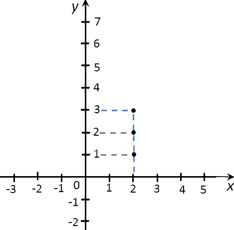
If we connect the obtained points of the graph of the function “x = 2”, we will get a straight line that is parallel to the “Oy” axis.

How to remember the rules for plotting functions of the form “y = 7” and “x = 2”

To plot functions of the form “y = 7” and “x = 2”, remember the following rule.

Constructing graphs of functions containing modules usually causes considerable difficulties for schoolchildren. However, everything is not so bad. It is enough to remember a few algorithms for solving such problems, and you can easily build a graph of even the most seemingly complex function. Let's figure out what kind of algorithms these are.

1. Plotting a graph of the function y = |f(x)|

Note that the set of function values y = |f(x)| : y ≥ 0. Thus, the graphs of such functions are always located entirely in the upper half-plane.

Plotting a graph of the function y = |f(x)| consists of the following simple four steps.

1) Carefully and carefully construct a graph of the function y = f(x).

2) Leave unchanged all points on the graph that are above or on the 0x axis.

3) Display the part of the graph that lies below the 0x axis symmetrically relative to the 0x axis.

Example 1. Draw a graph of the function y = |x 2 – 4x + 3|

1) We build a graph of the function y = x 2 – 4x + 3. Obviously, the graph of this function is a parabola. Let's find the coordinates of all points of intersection of the parabola with the coordinate axes and the coordinates of the vertex of the parabola.

x 2 – 4x + 3 = 0.

x 1 = 3, x 2 = 1.

Therefore, the parabola intersects the 0x axis at points (3, 0) and (1, 0).

y = 0 2 – 4 0 + 3 = 3.

Therefore, the parabola intersects the 0y axis at the point (0, 3).

Parabola vertex coordinates:

x in = -(-4/2) = 2, y in = 2 2 – 4 2 + 3 = -1.

Therefore, point (2, -1) is the vertex of this parabola.

Draw a parabola using the data obtained (Fig. 1)

2) The part of the graph lying below the 0x axis is displayed symmetrically relative to the 0x axis.

3) We get a graph of the original function ( rice. 2, shown as a dotted line).

2. Graphing the function y = f(|x|)

Note that functions of the form y = f(|x|) are even:

y(-x) = f(|-x|) = f(|x|) = y(x). This means that the graphs of such functions are symmetrical about the 0y axis.

Plotting a graph of the function y = f(|x|) consists of the following simple chain of actions.

1) Graph the function y = f(x).

2) Leave that part of the graph for which x ≥ 0, that is, the part of the graph located in the right half-plane.

3) Display the part of the graph specified in point (2) symmetrically to the 0y axis.

4) As the final graph, select the union of the curves obtained in points (2) and (3).

Example 2. Draw a graph of the function y = x 2 – 4 · |x| + 3

Since x 2 = |x| 2, then the original function can be rewritten in the following form: y = |x| 2 – 4 · |x| + 3. Now we can apply the algorithm proposed above.

1) We carefully and carefully build a graph of the function y = x 2 – 4 x + 3 (see also rice. 1).

2) We leave that part of the graph for which x ≥ 0, that is, the part of the graph located in the right half-plane.

3) Display the right side of the graph symmetrically to the 0y axis.

(Fig. 3).

Example 3. Draw a graph of the function y = log 2 |x|

We apply the scheme given above.

1) Build a graph of the function y = log 2 x (Fig. 4).

3. Plotting the function y = |f(|x|)|

Note that functions of the form y = |f(|x|)| are also even. Indeed, y(-x) = y = |f(|-x|)| = y = |f(|x|)| = y(x), and therefore, their graphs are symmetrical about the 0y axis. The set of values of such functions: y ≥ 0. This means that the graphs of such functions are located entirely in the upper half-plane.

To plot the function y = |f(|x|)|, you need to:

1) Carefully construct a graph of the function y = f(|x|).

2) Leave unchanged the part of the graph that is above or on the 0x axis.

3) Display the part of the graph located below the 0x axis symmetrically relative to the 0x axis.

4) As the final graph, select the union of the curves obtained in points (2) and (3).

Example 4. Draw a graph of the function y = |-x 2 + 2|x| – 1|.

1) Note that x 2 = |x| 2. This means that instead of the original function y = -x 2 + 2|x| - 1

you can use the function y = -|x| 2 + 2|x| – 1, since their graphs coincide.

We build a graph y = -|x| 2 + 2|x| – 1. For this we use algorithm 2.

a) Graph the function y = -x 2 + 2x – 1 (Fig. 6).

b) We leave that part of the graph that is located in the right half-plane.

c) We display the resulting part of the graph symmetrically to the 0y axis.

d) The resulting graph is shown in the dotted line in the figure (Fig. 7).

2) There are no points above the 0x axis; we leave the points on the 0x axis unchanged.

3) The part of the graph located below the 0x axis is displayed symmetrically relative to 0x.

4) The resulting graph is shown in the figure with a dotted line (Fig. 8).

Example 5. Graph the function y = |(2|x| – 4) / (|x| + 3)|

1) First you need to plot the function y = (2|x| – 4) / (|x| + 3). To do this, we return to Algorithm 2.

a) Carefully plot the function y = (2x – 4) / (x + 3) (Fig. 9).

Note that this function is fractional linear and its graph is a hyperbola. To plot a curve, you first need to find the asymptotes of the graph. Horizontal – y = 2/1 (the ratio of the coefficients of x in the numerator and denominator of the fraction), vertical – x = -3.

2) We will leave that part of the graph that is above the 0x axis or on it unchanged.

3) The part of the graph located below the 0x axis will be displayed symmetrically relative to 0x.

4) The final graph is shown in the figure (Fig. 11).

blog.site, when copying material in full or in part, a link to the original source is required.

A function graph is a visual representation of the behavior of a function on a coordinate plane. Graphs help you understand various aspects of a function that cannot be determined from the function itself. You can build graphs of many functions, and each of them will be given a specific formula. The graph of any function is built using a specific algorithm (if you have forgotten the exact process of graphing a specific function).

Steps

Graphing a Linear Function

Determine whether the function is linear. The linear function is given by a formula of the form F (x) = k x + b (\displaystyle F(x)=kx+b) or y = k x + b (\displaystyle y=kx+b)(for example, ), and its graph is a straight line. Thus, the formula includes one variable and one constant (constant) without any exponents, root signs, or the like. If a function of a similar type is given, it is quite simple to plot a graph of such a function. Here are other examples of linear functions:

Use a constant to mark a point on the Y axis. The constant (b) is the “y” coordinate of the point of intersection of the graph with the Y axis. That is, it is a point whose “x” coordinate is equal to 0. Thus, if x = 0 is substituted into the formula, then y = b (constant). In our example y = 2 x + 5 (\displaystyle y=2x+5) the constant is equal to 5, that is, the point of intersection with the Y axis has coordinates (0.5). Plot this point on the coordinate plane.

Find the slope of the line. It is equal to the multiplier of the variable. In our example y = 2 x + 5 (\displaystyle y=2x+5) with the variable “x” there is a factor of 2; thus, the slope coefficient is equal to 2. The slope coefficient determines the angle of inclination of the straight line to the X axis, that is, the greater the slope coefficient, the faster the function increases or decreases.

Write the slope as a fraction. The angular coefficient is equal to the tangent of the angle of inclination, that is, the ratio of the vertical distance (between two points on a straight line) to the horizontal distance (between the same points). In our example, the slope is 2, so we can state that the vertical distance is 2 and the horizontal distance is 1. Write this as a fraction: 2 1 (\displaystyle (\frac (2)(1))).

If the slope is negative, the function is decreasing.

From the point where the straight line intersects the Y axis, plot a second point using vertical and horizontal distances. A linear function can be graphed using two points. In our example, the intersection point with the Y axis has coordinates (0.5); From this point, move 2 spaces up and then 1 space to the right. Mark a point; it will have coordinates (1,7). Now you can draw a straight line.

Using a ruler, draw a straight line through two points. To avoid mistakes, find the third point, but in most cases the graph can be plotted using two points. Thus, you have plotted a linear function.

Plotting points on the coordinate plane
1. Define a function. The function is denoted as f(x). All possible values of the variable "y" are called the domain of the function, and all possible values of the variable "x" are called the domain of the function. For example, consider the function y = x+2, namely f(x) = x+2.
  
  Draw two intersecting perpendicular lines. The horizontal line is the X axis. The vertical line is the Y axis.
  
  Label the coordinate axes. Divide each axis into equal segments and number them. The intersection point of the axes is 0. For the X axis: positive numbers are plotted to the right (from 0), and negative numbers to the left. For the Y axis: positive numbers are plotted on top (from 0), and negative numbers on the bottom.
  
  Find the values of "y" from the values of "x". In our example, f(x) = x+2. Substitute specific x values into this formula to calculate the corresponding y values. If given a complex function, simplify it by isolating the “y” on one side of the equation.
  - -1: -1 + 2 = 1
  - 0: 0 +2 = 2
  - 1: 1 + 2 = 3
2. Plot the points on the coordinate plane. For each pair of coordinates, do the following: find the corresponding value on the X axis and draw a vertical line (dotted); find the corresponding value on the Y axis and draw a horizontal line (dashed line). Mark the intersection point of the two dotted lines; thus, you have plotted a point on the graph.
  
  Erase the dotted lines. Do this after plotting all the points on the graph on the coordinate plane. Note: the graph of the function f(x) = x is a straight line passing through the coordinate center [point with coordinates (0,0)]; the graph f(x) = x + 2 is a line parallel to the line f(x) = x, but shifted upward by two units and therefore passing through the point with coordinates (0,2) (because the constant is 2).
Graphing a Complex Function